
Berkas:Bloop locations.png
Ukuran pratayang ini: 600 × 600 piksel. Resolusi lainnya: 240 × 240 piksel | 480 × 480 piksel | 768 × 768 piksel | 1.024 × 1.024 piksel | 2.048 × 2.048 piksel | 3.000 × 3.000 piksel.
Ukuran asli (3.000 × 3.000 piksel, ukuran berkas: 7,74 MB, tipe MIME: image/png)
Ringkasan
| Deskripsi |
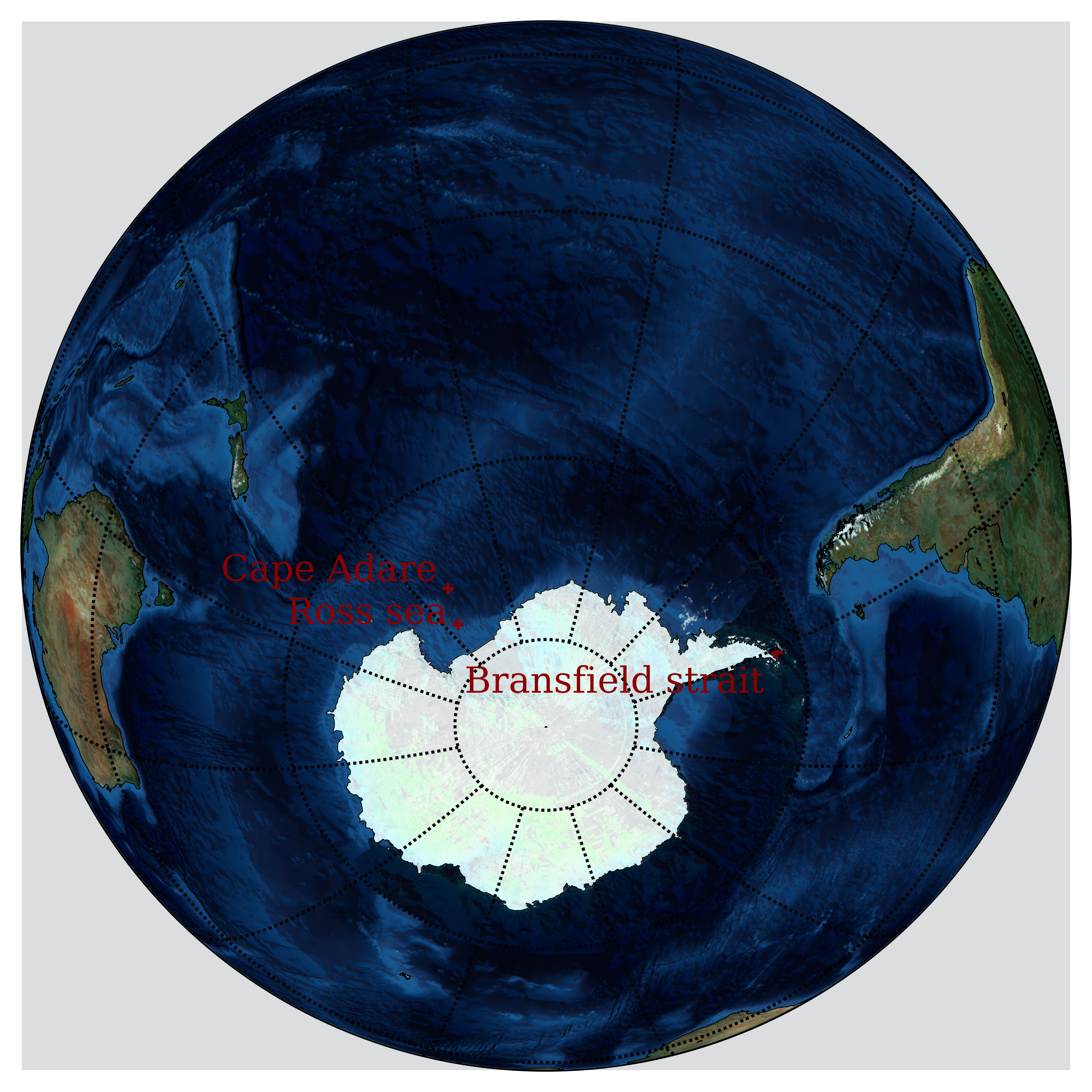
English: Possible locations of the Bloop, an ultra-low frequency and extremely powerful underwater sound detected by the U.S. National Oceanic and Atmospheric Administration (NOAA) in 1997. |
| Tanggal | |
| Sumber | Karya sendiri |
| Pembuat | Nojhan |
| PNG genesis |
Source code
This image has been generated by the following source code in Python:
Python code
| source code |
|---|
print "import modules...",
import sys
sys.stdout.flush()
import pickle
from mpl_toolkits.basemap import Basemap, shiftgrid, cm
import matplotlib
import matplotlib.pyplot as plt
import numpy as np
from netCDF4 import Dataset
print "ok"

# Lovecraft: 47:9'S 126:43'W
# lovecraft_lat = -47.9
# lovecraft_lon = -126.43

# August Derleth: 49:51'S 128:34'W
# derleth_lat = -49.51
# derleth_lon = -128.34

# Nemo point: 48:52.6'S 123:23.6'W
# nemo_lat = -48.526
# nemo_lon = -123.236

# The Bloop:
bransfield_strait_lat=-63
bransfield_strait_lon=-59
ross_sea_lat = -75
ross_sea_lon = -175
cape_adare_lat = -71.17
cape_adare_lon = -170.14

mid_lat = np.mean((bransfield_strait_lat,ross_sea_lat,cape_adare_lat))
mid_lon = np.mean((bransfield_strait_lon,ross_sea_lon,cape_adare_lon))


# Not necessary, because the default projection is ortho,
# but can be useful if you want another one.
def equi(m, centerlon, centerlat, radius, *args, **kwargs):
    """
    Drawing circles of a given radius around any point on earth, given the current projection.
    http://www.geophysique.be/2011/02/20/matplotlib-basemap-tutorial-09-drawing-circles/
    """
    glon1 = centerlon
    glat1 = centerlat
    X = []
    Y = []
    for azimuth in range(0, 360):
        glon2, glat2, baz = shoot(glon1, glat1, azimuth, radius)
        X.append(glon2)
        Y.append(glat2)
    X.append(X[0])
    Y.append(Y[0])

    #m.plot(X,Y,**kwargs) #Should work, but doesn't...
    X,Y = m(X,Y)
    plt.plot(X,Y,**kwargs)


def shoot(lon, lat, azimuth, maxdist=None):
    """Shooter Function
    Plotting great circles with Basemap, but knowing only the longitude,
    latitude, the azimuth and a distance. Only the origin point is known.
    Original javascript on http://williams.best.vwh.net/gccalc.htm
    Translated to python by Thomas Lecocq :
    http://www.geophysique.be/2011/02/19/matplotlib-basemap-tutorial-08-shooting-great-circles/
    """
    glat1 = lat * np.pi / 180.
    glon1 = lon * np.pi / 180.
    s = maxdist / 1.852
    faz = azimuth * np.pi / 180.

    EPS= 0.00000000005
    if ((np.abs(np.cos(glat1))<EPS) and not (np.abs(np.sin(faz))<EPS)):
        alert("Only N-S courses are meaningful, starting at a pole!")

    a=6378.13/1.852
    f=1/298.257223563
    r = 1 - f
    tu = r * np.tan(glat1)
    sf = np.sin(faz)
    cf = np.cos(faz)
    if (cf==0):
        b=0.
    else:
        b=2. * np.arctan2 (tu, cf)

    cu = 1. / np.sqrt(1 + tu * tu)
    su = tu * cu
    sa = cu * sf
    c2a = 1 - sa * sa
    x = 1. + np.sqrt(1. + c2a * (1. / (r * r) - 1.))
    x = (x - 2.) / x
    c = 1. - x
    c = (x * x / 4. + 1.) / c
    d = (0.375 * x * x - 1.) * x
    tu = s / (r * a * c)
    y = tu
    c = y + 1
    while (np.abs (y - c) > EPS):

        sy = np.sin(y)
        cy = np.cos(y)
        cz = np.cos(b + y)
        e = 2. * cz * cz - 1.
        c = y
        x = e * cy
        y = e + e - 1.
        y = (((sy * sy * 4. - 3.) * y * cz * d / 6. + x) *
              d / 4. - cz) * sy * d + tu

    b = cu * cy * cf - su * sy
    c = r * np.sqrt(sa * sa + b * b)
    d = su * cy + cu * sy * cf
    glat2 = (np.arctan2(d, c) + np.pi) % (2*np.pi) - np.pi
    c = cu * cy - su * sy * cf
    x = np.arctan2(sy * sf, c)
    c = ((-3. * c2a + 4.) * f + 4.) * c2a * f / 16.
    d = ((e * cy * c + cz) * sy * c + y) * sa
    glon2 = ((glon1 + x - (1. - c) * d * f + np.pi) % (2*np.pi)) - np.pi

    baz = (np.arctan2(sa, b) + np.pi) % (2 * np.pi)

    glon2 *= 180./np.pi
    glat2 *= 180./np.pi
    baz *= 180./np.pi

    return (glon2, glat2, baz)


print "read in etopo5 topography/bathymetry"
url = 'http://ferret.pmel.noaa.gov/thredds/dodsC/data/PMEL/etopo5.nc'
etopodata = Dataset(url)

print "get data"

def topopickle(etopodata,name):
    import sys
    print "\t"+name+"...",
    sys.stdout.flush()
    filename = "rlyeh_"+name+".pickle"
    try:
        with open(filename,"r") as fd:
            print "load...",
            var = pickle.load(fd)
    except IOError:
        print "copy...",
        var = etopodata.variables[name][:]
        with open(filename,"w") as fd:
            print "dump...",
            pickle.dump(var,fd)
    print "ok"
    return var

topoin = topopickle(etopodata,"ROSE")
lons   = topopickle(etopodata,"ETOPO05_X")
lats   = topopickle(etopodata,"ETOPO05_Y")
print "shift data so lons go from -180 to 180 instead of 20 to 380...",
sys.stdout.flush()
topoin,lons = shiftgrid(180.,topoin,lons,start=False)
print "ok"


# create the figure and axes instances.
fig = plt.figure()
ax = fig.add_axes([0.1,0.1,0.8,0.8])

print "setup basemap"
# set up orthographic m projection with
# perspective of satellite looking down at 50N, 100W.
# use low resolution coastlines.
m = Basemap(projection='ortho',lat_0=mid_lat,lon_0=mid_lon,resolution='l')
m.bluemarble()

# Generic Mapping Tools colormaps:
# GMT_drywet, GMT_gebco, GMT_globe, GMT_haxby GMT_no_green, GMT_ocean, GMT_polar,
# GMT_red2green, GMT_relief, GMT_split, GMT_wysiwyg

print "transform to nx x ny regularly spaced native projection grid"
# step=5000.
step=10000.
nx = int((m.xmax-m.xmin)/step)+1; ny = int((m.ymax-m.ymin)/step)+1
topodat = m.transform_scalar(topoin,lons,lats,nx,ny)

print "plot topography/bathymetry as shadows"
from matplotlib.colors import LightSource
ls = LightSource(azdeg = 45, altdeg = 220, hsv_min_val=0.0, hsv_max_val=1.0,
        hsv_min_sat=0.0, hsv_max_sat=1.0)
# convert data to rgb array including shading from light source.
# (must specify color m)
rgb = ls.shade(topodat, cm.GMT_ocean)
im = m.imshow(rgb, alpha=0.15)

print "draw coastlines, country boundaries, fill continents"
m.drawcoastlines(linewidth=0.25)
# draw the edge of the map projection region
m.drawmapboundary(fill_color='white')
# draw lat/lon grid lines every 30 degrees.
m.drawmeridians(np.arange(  0,360,30), color="black" )
m.drawparallels(np.arange(-90,90 ,30), color="black" )

print "draw points"
psize=5
font = {'family' : 'serif',
        'weight' : 'normal',
        'size'   : 12}
matplotlib.rc('font', **font)

# x,y = m( lovecraft_lon, lovecraft_lat )
# m.scatter(x,y,psize,marker='o', color='white')
# plt.text(x+50000,y+50000+50000, "Lovecraft", color='white')
#
# x,y = m( derleth_lon, derleth_lat )
# m.scatter(x,y,psize,marker='o',color='white')
# plt.text(x+50000-120000,y+50000, "Derleth", color='white', horizontalalignment="right")

# x,y = m( nemo_lon, nemo_lat )
# m.scatter(x,y,psize*3,marker='+',color='#555555')
# plt.text(x+50000+50000,y+50000-80000, "Nemo", color="#555555", verticalalignment="top")
#
# equi(m, nemo_lon, nemo_lat, radius=2688, color="#555555" )

pcolor="darkred"
offset=150000

x,y = m( bransfield_strait_lon, bransfield_strait_lat )
m.scatter(x,y,psize*3,marker='+',color=pcolor)
plt.text(x-offset,y-offset, "Bransfield strait", color=pcolor,
        horizontalalignment="right", verticalalignment="top")

x,y = m( ross_sea_lon, ross_sea_lat )
m.scatter(x,y,psize*3,marker='+',color=pcolor)
plt.text(x-offset,y, "Ross sea", color=pcolor,
        horizontalalignment="right", verticalalignment="bottom")

x,y = m( cape_adare_lon, cape_adare_lat )
m.scatter(x,y,psize*3,marker='+',color=pcolor)
plt.text(x-offset,y, "Cape Adare", color=pcolor,
        horizontalalignment="right", verticalalignment="bottom")

plt.savefig("Bloop_locations.png", dpi=600, bbox_inches='tight')
# plt.show()
|
Lisensi
Saya, pemilik hak cipta dari karya ini, dengan ini menerbitkan berkas ini di bawah ketentuan berikut:
Berkas on ipartandoan sian on Creative Commons Attribution-Share Alike 3.0 Unported partadoan.
- Anda diizinkan:
- untuk berbagi – untuk menyalin, mendistribusikan dan memindahkan karya ini
- untuk menggubah – untuk mengadaptasi karya ini
- Berdasarkan ketentuan berikut:
- atribusi – Anda harus mencantumkan atribusi yang sesuai, memberikan pranala ke lisensi, dan memberi tahu bila ada perubahan. Anda dapat melakukannya melalui cara yang Anda inginkan, namun tidak menyatakan bahwa pemberi lisensi mendukung Anda atau penggunaan Anda.
- berbagi serupa – Apabila Anda menggubah, mengubah, atau membuat turunan dari materi ini, Anda harus menyebarluaskan kontribusi Anda di bawah lisensi yang sama seperti lisensi pada materi asli.
Riwayat berkas
Klik pada tanggal/waktu untuk melihat berkas ini pada saat tersebut.
| Tanggal/Waktu | Miniatur | Dimensi | Pengguna | Komentar | |
|---|---|---|---|---|---|
| terkini | 12 Februari 2013 21.46 | | 3.000 × 3.000 (7,74 MB) | Nojhan | User created page with UploadWizard |
Penggunaan berkas
Halaman berikut menggunakan berkas ini:
Penggunaan berkas global
Wiki lain berikut menggunakan berkas ini: